Chemistry Tutorial
This tutorial shows how to compute chemistry with chemcat under different assumptions for temperature, metallicity, and custom elemental abundances.
You can also find this tutorial as a Python scrip here or as a jupyter notebook here.
Basic run
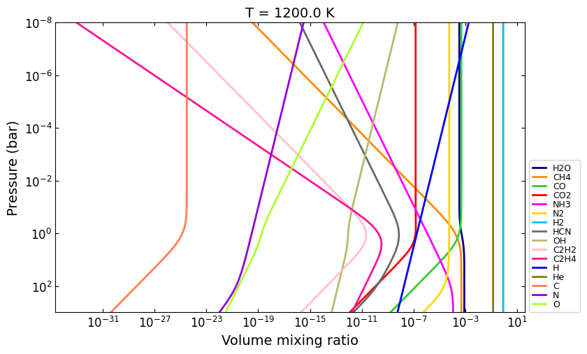
chemcat is an object-oriented code that keeps all the thermochemical properties in place. In it most basic usage, all it requres is a pressure-temperature profile and a list of species.
This creates a chemical network assuming solar elemental composition and a simple CHNO compostion (taking values from Asplund et al. 2021):
[1]:
# Let's start importing the necessary modules
import chemcat as cat
import chemcat.utils as u
import numpy as np


nlayers = 81
temperature = np.tile(1200.0, nlayers)
pressure = np.logspace(-8, 3, nlayers)
molecules = 'H2O CH4 CO CO2 NH3 N2 H2 HCN OH C2H2 C2H4 H He C N O'.split()

net = cat.Network(pressure, temperature, molecules)

# To compute thermochemical equilibrium abundances, run this method:
vmr = net.thermochemical_equilibrium()

# and plot the results:
title = f'T = {temperature[0]} K'
ax = u.plot_vmr(pressure, vmr, net.species, title=title, fignum=10)
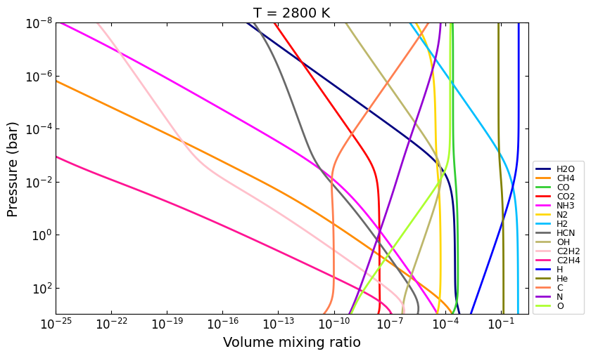
Update temperature
[2]:
# Simply, provide a new temperature profile in the call:
temp_2800K = np.tile(2800, nlayers)
vmr = net.thermochemical_equilibrium(temperature=temp_2800K)

title = f'T = {temp_2800K[0]} K'
vmr_range = (1e-25, 3)
ax = u.plot_vmr(pressure, vmr, net.species, vmr_range=vmr_range, title=title, fignum=20)
Object’s data
The net object contains all the physical data of the atmosphere, which you can query at any point:
[3]:
print(f'Pressure profile (bar):\n{net.pressure}')
print(f'\nTemperature profile (kelvin):\n{net.temperature}')

print(f'\nElemental composition:\n{net.elements}')
print('\nElemental abundances (normalized to H_abundance==1.0)'
      f'\n(same order as in the array above):\n{net.element_rel_abundance}')
print(f'\nElemental composition source:\n{net.element_file}')

print(f'\n\nMolecular composition:\n{net.species}')
print(f'Source for each species thermochemical data:\n{net.provenance}')
print(
    '\nStoichiometric values matrix for each species:'
    '\n(order of values goes according to order of elements and species arrays)'
    f'\n{net.stoich_vals}')
Pressure profile (bar):
[1.00000000e-08 1.37246096e-08 1.88364909e-08 2.58523484e-08
 3.54813389e-08 4.86967525e-08 6.68343918e-08 9.17275935e-08
 1.25892541e-07 1.72782598e-07 2.37137371e-07 3.25461783e-07
 4.46683592e-07 6.13055792e-07 8.41395142e-07 1.15478198e-06
 1.58489319e-06 2.17520403e-06 2.98538262e-06 4.09732110e-06
 5.62341325e-06 7.71791516e-06 1.05925373e-05 1.45378439e-05
 1.99526231e-05 2.73841963e-05 3.75837404e-05 5.15822165e-05
 7.07945784e-05 9.71627952e-05 1.33352143e-04 1.83020611e-04
 2.51188643e-04 3.44746607e-04 4.73151259e-04 6.49381632e-04
 8.91250938e-04 1.22320712e-03 1.67880402e-03 2.30409298e-03
 3.16227766e-03 4.34010264e-03 5.95662144e-03 8.17523038e-03
 1.12201845e-02 1.53992653e-02 2.11348904e-02 2.90068120e-02
 3.98107171e-02 5.46386550e-02 7.49894209e-02 1.02920053e-01
 1.41253754e-01 1.93865264e-01 2.66072506e-01 3.65174127e-01
 5.01187234e-01 6.87859912e-01 9.44060876e-01 1.29568670e+00
 1.77827941e+00 2.44061907e+00 3.34965439e+00 4.59726989e+00
 6.30957344e+00 8.65964323e+00 1.18850223e+01 1.63117291e+01
 2.23872114e+01 3.07255737e+01 4.21696503e+01 5.78761988e+01
 7.94328235e+01 1.09018449e+02 1.49623566e+02 2.05352503e+02
 2.81838293e+02 3.86812055e+02 5.30884444e+02 7.28618175e+02
 1.00000000e+03]

Temperature profile (kelvin):
[2800 2800 2800 2800 2800 2800 2800 2800 2800 2800 2800 2800 2800 2800
 2800 2800 2800 2800 2800 2800 2800 2800 2800 2800 2800 2800 2800 2800
 2800 2800 2800 2800 2800 2800 2800 2800 2800 2800 2800 2800 2800 2800
 2800 2800 2800 2800 2800 2800 2800 2800 2800 2800 2800 2800 2800 2800
 2800 2800 2800 2800 2800 2800 2800 2800 2800 2800 2800 2800 2800 2800
 2800 2800 2800 2800 2800 2800 2800 2800 2800 2800 2800]

Elemental composition:
['C' 'H' 'He' 'N' 'O']

Elemental abundances (normalized to H_abundance==1.0)
(same order as in the array above):
[2.88403150e-04 1.00000000e+00 8.20351544e-02 6.76082975e-05
 4.89778819e-04]

Elemental composition source:
/home/pcubillos/Dropbox/IWF/projects/2022_chemcat/chemcat/chemcat/data/asplund_2021_solar_abundances.dat


Molecular composition:
['H2O' 'CH4' 'CO' 'CO2' 'NH3' 'N2' 'H2' 'HCN' 'OH' 'C2H2' 'C2H4' 'H' 'He'
 'C' 'N' 'O']
Source for each species thermochemical data:
['janaf' 'janaf' 'janaf' 'janaf' 'janaf' 'janaf' 'janaf' 'janaf' 'janaf'
 'janaf' 'janaf' 'janaf' 'janaf' 'janaf' 'janaf' 'janaf']

Stoichiometric values matrix for each species:
(order of values goes according to order of elements and species arrays)
[[0 2 0 0 1]
 [1 4 0 0 0]
 [1 0 0 0 1]
 [1 0 0 0 2]
 [0 3 0 1 0]
 [0 0 0 2 0]
 [0 2 0 0 0]
 [1 1 0 1 0]
 [0 1 0 0 1]
 [2 2 0 0 0]
 [2 4 0 0 0]
 [0 1 0 0 0]
 [0 0 1 0 0]
 [1 0 0 0 0]
 [0 0 0 1 0]
 [0 0 0 0 1]]
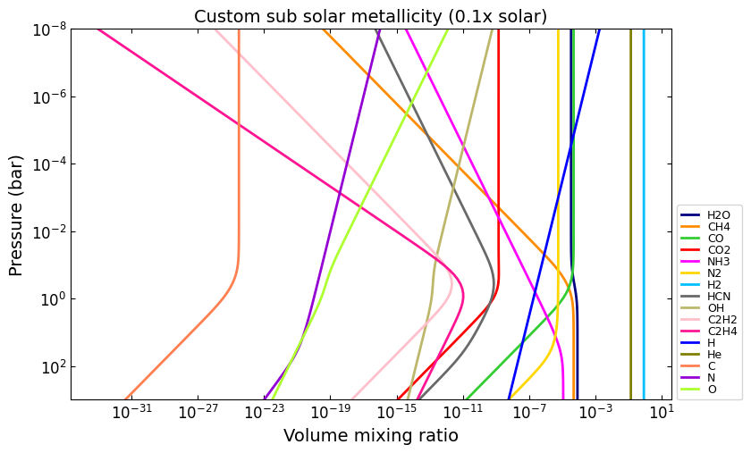
Custom compositions
There are a few alternatives evaluate thermochemical equilibrium for different compositions
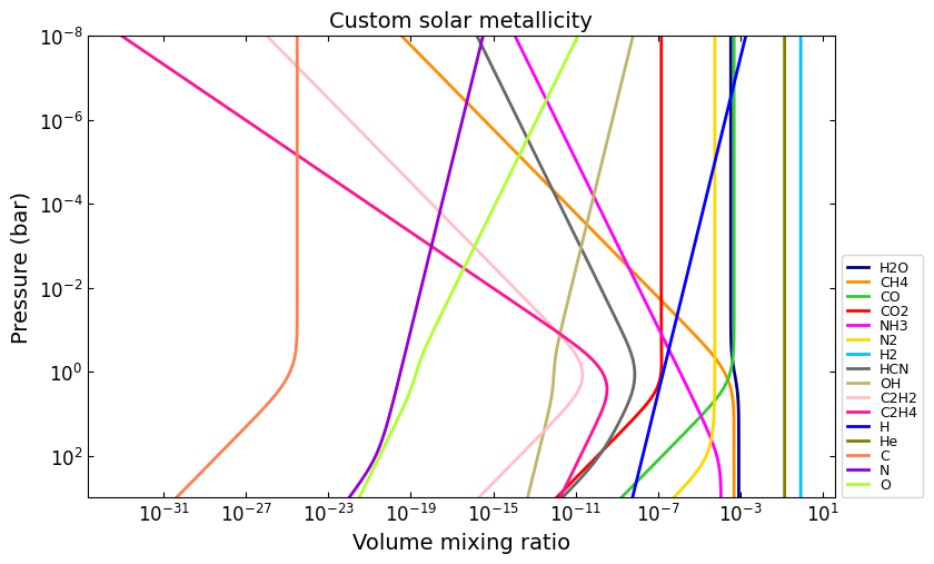
Custom metallicity
Use the metallicity argument to set a custom metallicity relative to solar (in dex units)
[4]:
# E.g., solar metallicity (default):
net = cat.Network(pressure, temperature, molecules)
vmr_custom_solar = net.thermochemical_equilibrium(
metallicity=0.0,
)
# e.g, 0.1x solar metallicity:
vmr_custom_sub_solar = net.thermochemical_equilibrium(
metallicity=-1.0,
)
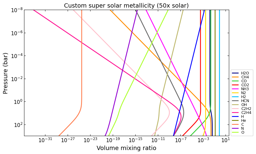
# e.g, 50x solar metallicity:
metallicity = np.log10(50.0)
vmr_custom_super_solar = net.thermochemical_equilibrium(
metallicity=metallicity,
)
# And plot the results:
title = 'Custom sub solar metallicity (0.1x solar)'
ax = u.plot_vmr(pressure, vmr_custom_sub_solar, net.species, title=title, fignum=30)
title = 'Custom solar metallicity'
ax = u.plot_vmr(pressure, vmr_custom_solar, net.species, title=title, fignum=31)
title = 'Custom super solar metallicity (50x solar)'
ax = u.plot_vmr(pressure, vmr_custom_super_solar, net.species, title=title, fignum=32)
Note that once you modify a physical property, it stays modified until you re-set it again:
[5]:
print(f'[M/H] = {net.metallicity:.2f}')
print(f'Elemental abundances:\n{net.element_rel_abundance}')

# You can modify the properties directly:
net.metallicity = 0.0
print(f'\n[M/H] = {net.metallicity}')
print(f'Elemental abundances:\n{net.element_rel_abundance}')

# Or, you can modify the properties via a call:
# e.g, 50x solar:
vmr_custom_super_solar = net.thermochemical_equilibrium(
    metallicity=np.log10(50.0),
)
print(f'\n[M/H] = {net.metallicity:.2f}')
print(f'Elemental abundances:\n{net.element_rel_abundance}')
[M/H] = 1.70
Elemental abundances:
[0.01442016 1.         0.08203515 0.00338041 0.02448894]

[M/H] = 0.0
Elemental abundances:
[2.88403150e-04 1.00000000e+00 8.20351544e-02 6.76082975e-05
 4.89778819e-04]

[M/H] = 1.70
Elemental abundances:
[0.01442016 1.         0.08203515 0.00338041 0.02448894]
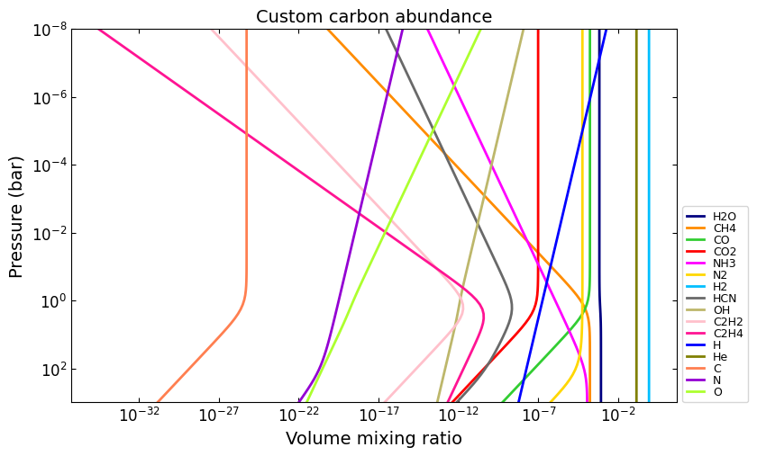
Custom elemental abundances
Use the e_abundances argument to set custom elemental abundances as a dictionary: (values in dex units, relative to H=12.0). Note that e_abundances override values modified by metallicity.
[6]:
# E.g., set carbon abundance to 10^-4
e_abundances = {
'C': 8.0,
}
vmr_custom_abundance1 = net.thermochemical_equilibrium(
metallicity=0.0,
e_abundances=e_abundances,
)
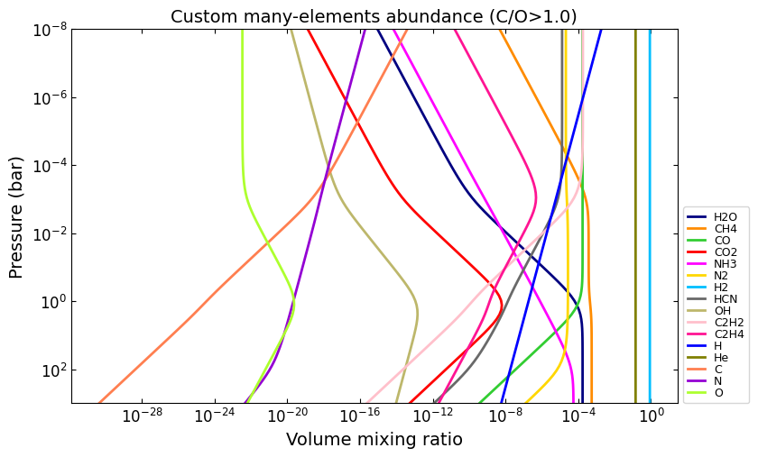
# You can set values for as many elements as you want, e.g.:
e_abundances = {
'C': 8.5,
'N': 7.5,
'O': 8.0,
}
vmr_custom_abundance2 = net.thermochemical_equilibrium(
e_abundances=e_abundances,
)
# And plot the results:
title = 'Custom carbon abundance'
ax = u.plot_vmr(pressure, vmr_custom_abundance1, net.species, title=title, fignum=33)
title = 'Custom many-elements abundance (C/O>1.0)'
ax = u.plot_vmr(pressure, vmr_custom_abundance2, net.species, title=title, fignum=34)
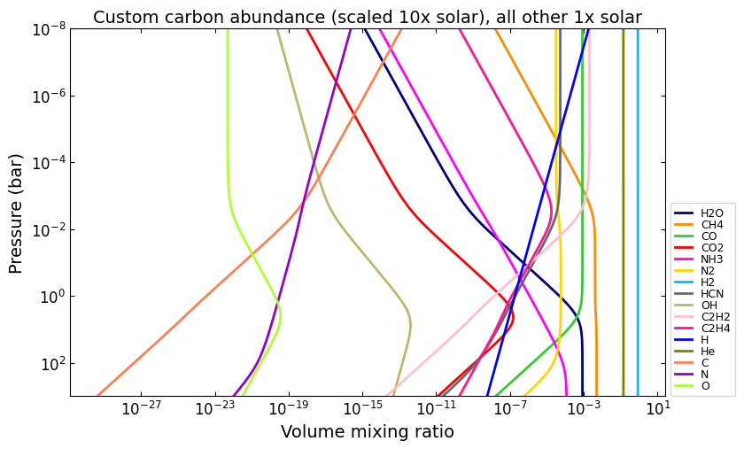
Custom solar ratios
Use the e_scale argument to set custom elemental abundances as a dictionary (values in dex units, relative to solar). Note that e_scale values override values modified by metallicity.
[7]:
# E.g., Set 10x solar carbon, 1x nitrogen, and 1x oxygen
e_scale = {
    'C': 1.0,
    'N': 0.0,
    'O': 0.0,
}

vmr_custom_scale_carbon = net.thermochemical_equilibrium(
    metallicity=0.0,
    e_abundances={},
    e_scale=e_scale,
)

# And plot the results:
title = 'Custom carbon abundance (scaled 10x solar), all other 1x solar'
ax = u.plot_vmr(pressure, vmr_custom_scale_carbon, net.species, title=title, fignum=35)
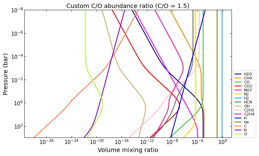
Custom elemental ratios
Use the e_ratio argument to set custom elemental abundances as a dictionary (values are not in dex units, relative to a second elemental abundance).
Note that the dictionary keys define the pair of elements separated by an underscore. Only the first element abundance is modified, and is scaled relative to the second element’s abundance.
[8]:
# E.g., set carbon abundance to 1.5x times the oxygen abundance:
e_ratio = {
    'C_O': 1.5,
}

vmr_custom_ratio = net.thermochemical_equilibrium(
    metallicity=0.0,
    e_abundances={},
    e_ratio=e_ratio,
)

# And plot the results:
title = 'Custom C/O abundance ratio (C/O = 1.5)'
ax = u.plot_vmr(pressure, vmr_custom_ratio, net.species, title=title, fignum=36)
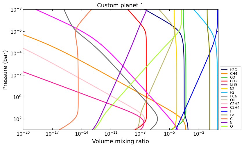
And you can combine all these properties at once:
[9]:
# Custom metallicity, C/O ratio, and temperatures:
# Hot, sub-solar (0.1x), C/O < 1.0:
temp_2000K = np.tile(2000.0, nlayers)
metal_sub_solar = -1.0
e_ratio = {
'C_O': 0.6,
}
vmr_custom1 = net.thermochemical_equilibrium(
temperature=temp_2000K,
metallicity=metal_sub_solar,
e_ratio=e_ratio,
)
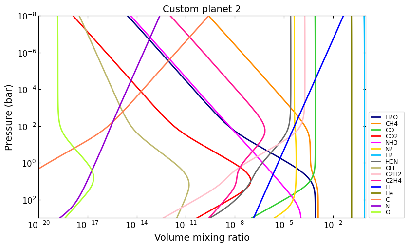
# Colder, super-solar (50x), and C/O > 1.0:
temp_1400K = np.tile(1400.0, nlayers)
metal_super_solar = np.log10(50.0)
e_ratio = {
'C_O': 1.5,
}
vmr_custom2 = net.thermochemical_equilibrium(
temperature=temp_1400K,
metallicity=metal_super_solar,
e_ratio=e_ratio,
)
# And plot the results:
vmr_range = (1e-20, 1)
title = 'Custom planet 1'
ax = u.plot_vmr(
pressure, vmr_custom1, net.species,
title=title, fignum=37, vmr_range=vmr_range,
)
title = 'Custom planet 2'
ax = u.plot_vmr(
pressure, vmr_custom2, net.species,
title=title, fignum=38, vmr_range=vmr_range,
)
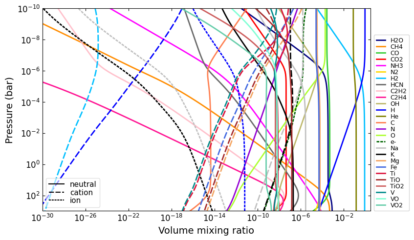
Charge conservation
Charge conservation is also available, ions are specified by species names followed by a
+or a-Normally, you always need to include an electron in the mix: ‘e-’
[10]:
nlayers = 81
temp = 2000.0
temperature = np.tile(temp, nlayers)
pressure = np.logspace(-10, 3, nlayers)

HCNO_neutrals = 'H2O CH4 CO CO2 NH3 N2 H2 HCN C2H2 C2H4 OH H He C N O'.split()
ions = 'e- H- H+ H2+ He+'.split()
alkali = 'Na Na- Na+ K K- K+'.split()
metals = 'Mg Mg+ Fe Fe+'.split()
metal_oxides = 'Ti TiO TiO2 Ti+ TiO+ V VO VO2 V+'.split()
molecules = (
    HCNO_neutrals
    + ions
    + alkali
    + metals
    + metal_oxides
)

net = cat.Network(pressure, temperature, molecules)
vmr = net.thermochemical_equilibrium()
vmr_range = (1e-30, 3)
ax = u.plot_vmr(pressure, vmr, net.species, vmr_range=vmr_range, fignum=40)